Optimizing PN parameters and fixing the BMS frame for NR waveform hybridizations

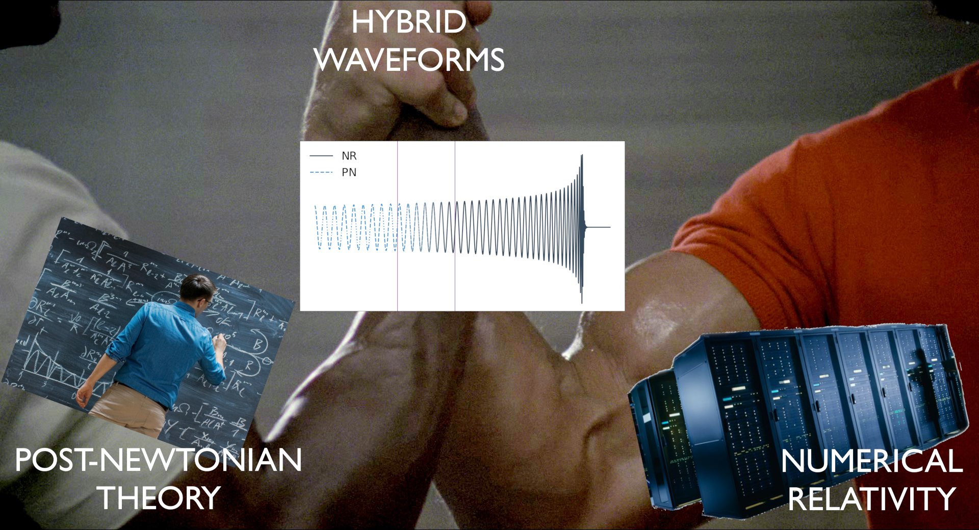
What are hybrid gravitational waveforms? In meme form:

Post-Newtonian       Numerical relativity
                 🤝
           Hybrid waveforms

Ok, but what does it actually mean? This new preprint [arXiv:2403.10278] was led by Caltech grad student Dongze Sun. Topics to cover:

• What is PN? What is NR? What is hybridization?
• What do you need to control in hybridization?
• You’re changing the masses/spins??
• Limitations we found

When solving the Einstein’s field equations of general relativity for a binary problem, we break down the space into separate regimes, where different tools are useful (figure courtesy of Leor Barack):

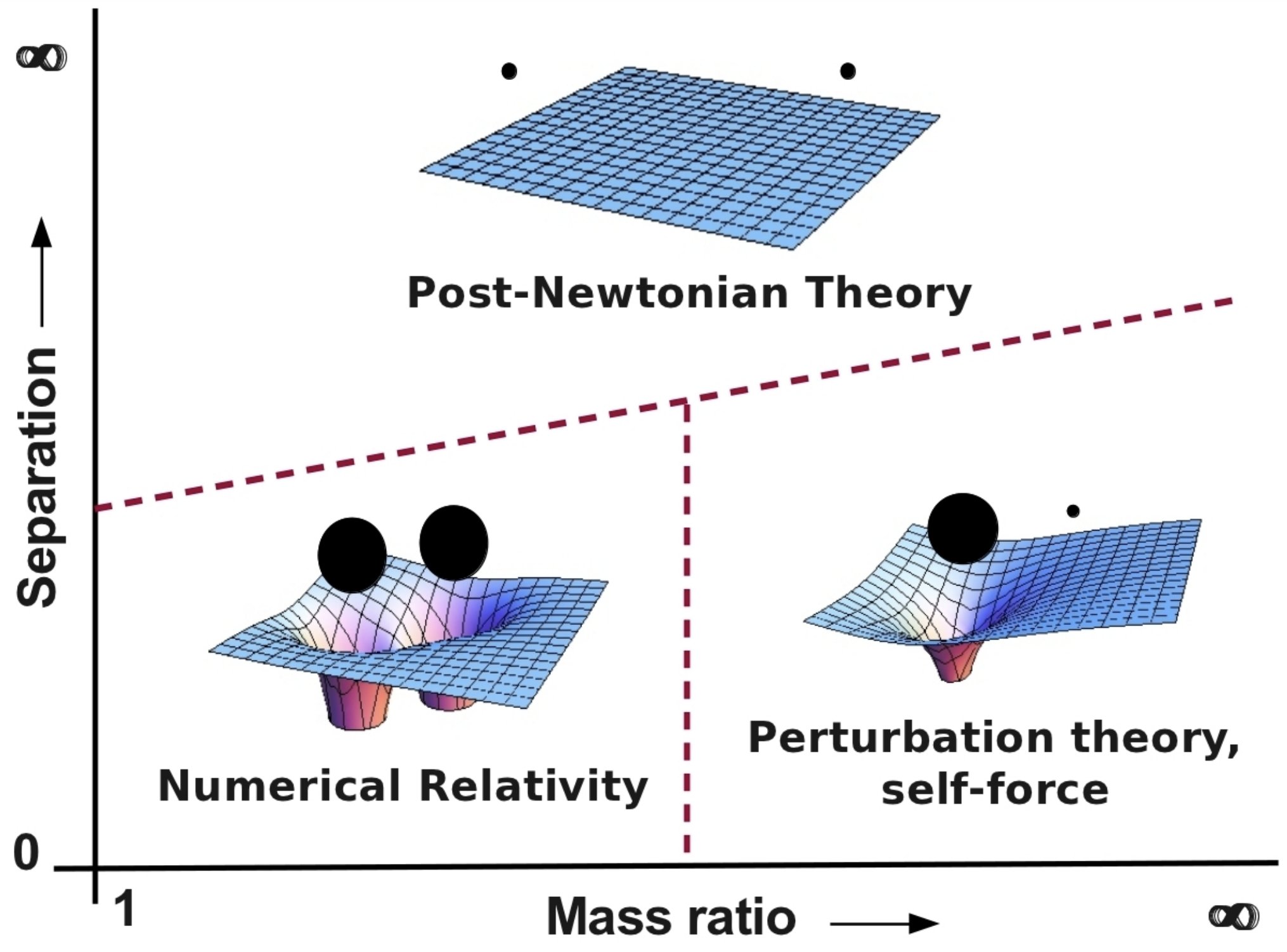
Post-Newtonian (PN) theory is the oldest, started by Einstein himself, and Lorentz+Droste way back in 1916. PN is valid when the bodies are widely separated, moving slowly, you stay “close to” Newtonian gravity. You do lots of integrals, getting analytical expressions:

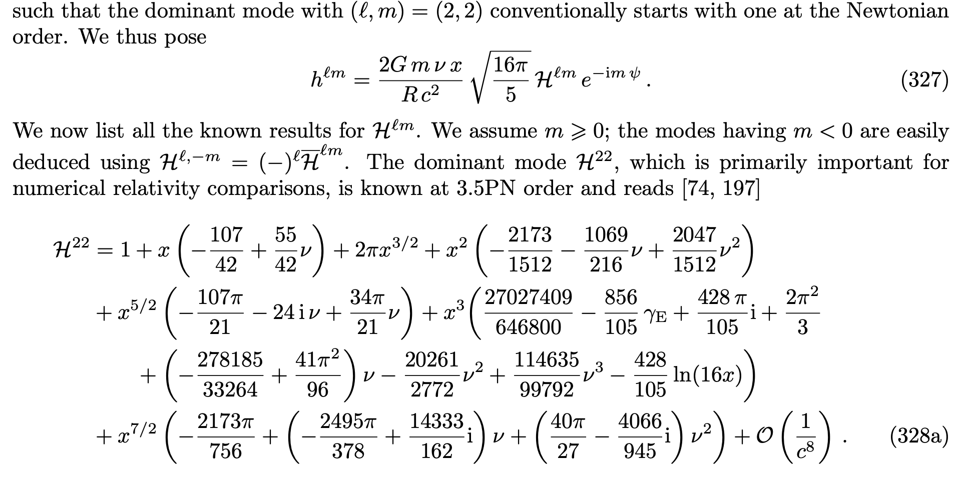
These expressions keep going on for pages… but PN breaks down when black holes get close enough and then merge. That’s why we need numerical relativity (NR).

Numerical relativity is the “ground truth” for waveforms that LIGO compares data against (including other waveform models like EOB and Phenom). In an ideal world, we would just use NR. But NR is inefficient when the bodies are far apart (or have a high mass ratio).

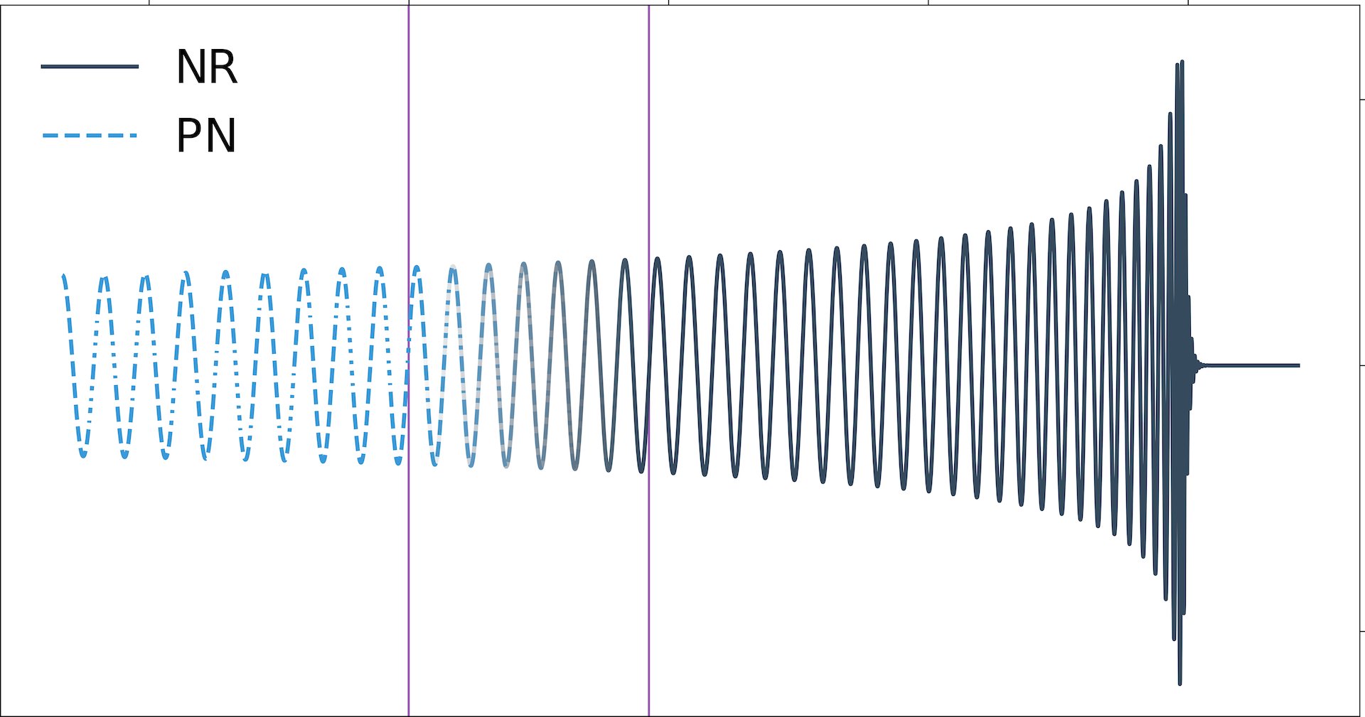
This is a problem if we want to compare against very long signals, like those coming from low-mass binaries. What’s the solutions? Hybridize! Hybridizing waveforms just means finding how to get them to smoothly agree in a “matching window”, then blending from one waveform (PN at early times) to the other (NR at late times).

How does hybridization work in practice? Well, in NR simulations compute some masses and spins from the black hole horizons (that’s a whole other story). Then you plug those masses and spins into PN and get a waveform, and align the two.

In the past, people hybridized with just one “mode” of the waveform, and all they did was shift the times and/or phase. But a gravitational waveform has an infinite number of modes. They should all get aligned, and there are more parameters to fiddle with. Ok, you say. I have one overall time shift, and one spatial rotation. That’s just 4 parameters. But you also need the PN/NR binaries to have the same center of momentum, and center of mass. Those all show up in gravitational waves! Is that it?

So far those are just the “Poincaré” transformations of Minkowski space. But curved spacetime is more complicated! It turns out that at “future null infinity,” there are an infinite number of “angle-dependent translations” to fix! What does that mean?

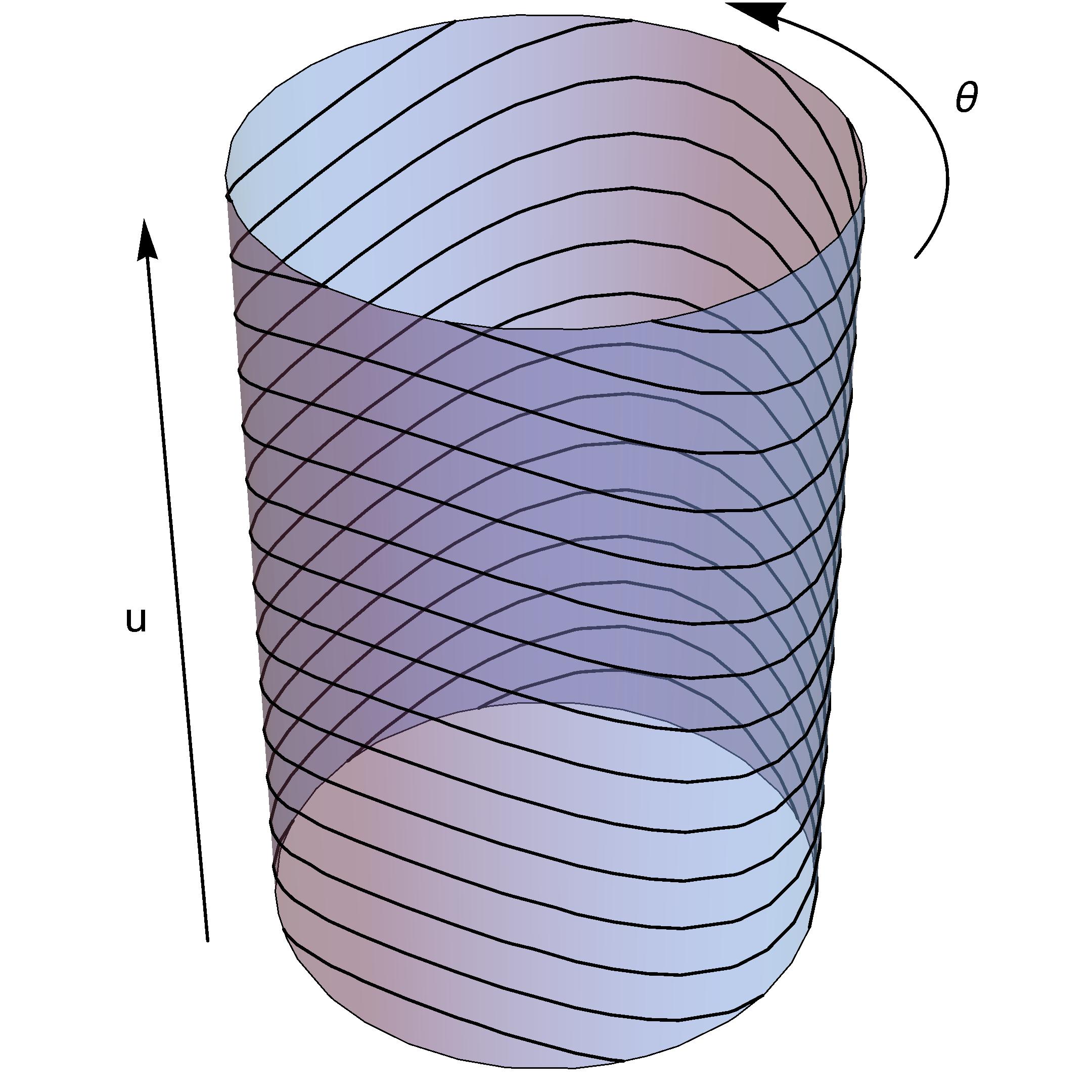
This is called the “BMS group,” after Bondi, van der Burg, Metzner, and Sachs (van der Burg seems to have been dropped from the initialism). Basically, because observers at future null infinity (“scri”) can’t synchronize their clocks, you can smoothly reslice the time function on scri. That’s called a supertranslation, which looks vaguely like this blue cylinder.

Ok, you say, I’ve got to fix the 10 Poincaré parameters and an infinite number of supertranslation freedoms (which in practice is 76 for us). But wait, there’s more! You still have to twiddle the masses and spins. Wait a second, didn’t we just say that we get the masses and spin from the numerical relativity simulations? Well yes, but actually no.

The problem is, the way masses and spins are defined in post-Newtonian theory is very different from how they’re defined in numerical relativity, and there’s actually no deep reason for them to agree. Basically, it’s the same parameter space, but with different coordinates:

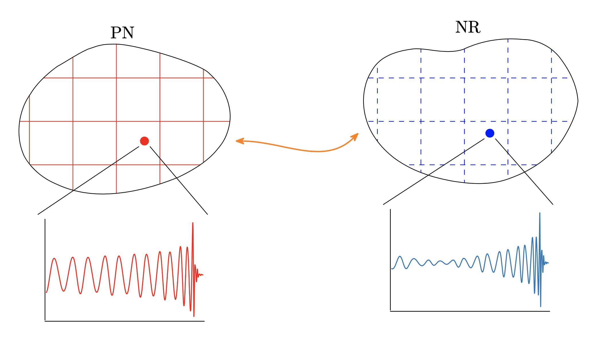
What we really need to do is let the observables tell us where we are in parameter space. The observables in this case are the gravitational waves! They have all the information about black hole masses and spins.

So, Dongze wrote lots of code that wraps this all up: within a matching window, fix all the Poincaré and BMS freedoms. Now twiddle the PN masses and spins (since the NR simulation is fixed). Then iterate, and soon, you’ve converged to the true PN+BMS parameters. It’s tricky!

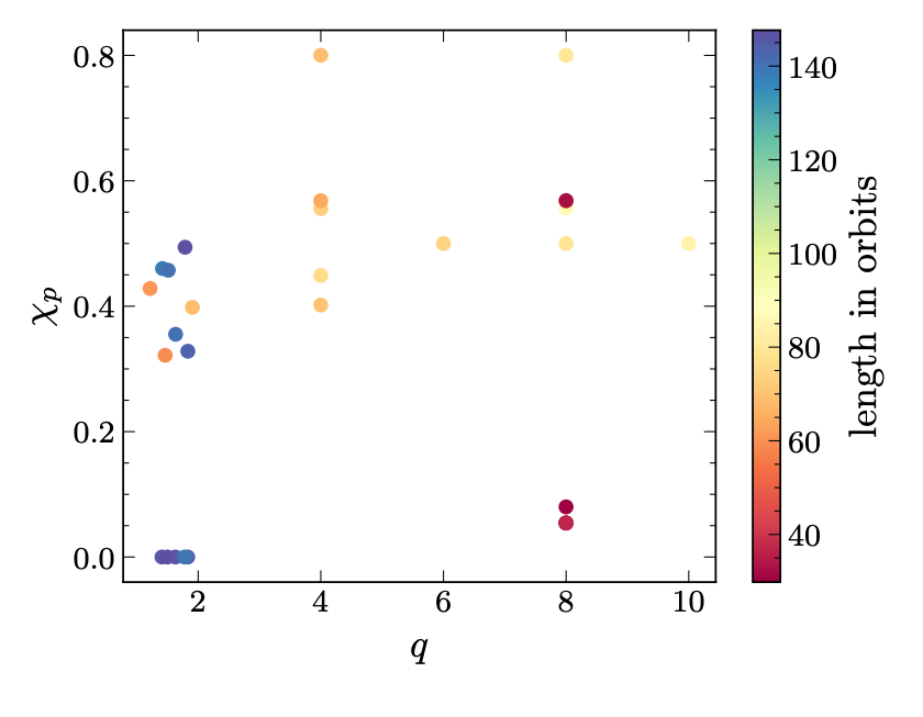
Most of the paper is characterizing what we learn from studying how this procedure works on 29 NR simulations that have mass ratios from 1-10, with spins up to 80% of max, that are precessing, and do between 60-100+ orbits. In units that relativists know, up to 10⁵M long!

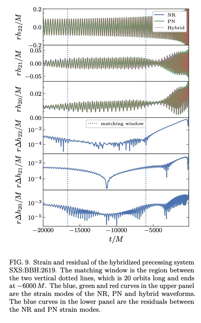
Below is the kind of thing you can get from Dongze’s code. Top three panels are different modes of the same waveform. The matching window is between the vertical lines. Optimizing gets BMS-transformed PN to agree with NR, with residuals in the bottom 3 panels.

What are the main things we learned?

• Fitting as above (varying PN and BMS params) is the “right” thing to do, but might result in over-fitting
• For non-precessing systems, we can do quite well. We’re limited by eccentricity.
• Precession is harder, PN needs to improve

What’s going on with eccentricity and precession? These are very important phenomena. A general orbit will be eccentric, but gravitational waves make it circularize as time goes on. That’s why most PN calculations have focused on quasicircular binaries.

Nature is more complicated, and we should have eccentricity. But still, most NR has also focused on trying to simulate quasicircular binaries. Our code SpEC does something called “eccentricity reduction” to make binaries as circular as possible. But it’s imperfect. There is still some residual eccentricity, but we’ve been trying to compare these NR waveforms against quasicircular PN waveforms. Even though the eccentricity might be tiny (say, \(10^{-5}\)), it still has a measurable effect on the waveform, and we aren’t trying to model it on the PN side of things. So, eccentricity is our dominant limitation for spin-aligned (non-precessing) systems.

Moving on to precession. When black hole spins are misaligned form the orbital angular momentum, the spins and the orbit all precess. This wobbling is a key signature to look for in the gravitational waves. It also makes the post-Newtonian calculations much harder! We found that more precession makes PN-NR agree less.

In fact, Dongze even calibrated a function that estimates how well PN and NR will agree as a function of the amount of precession. You can use this function to figure out how long your NR simulation should be in order to hybridize at a certain precision.

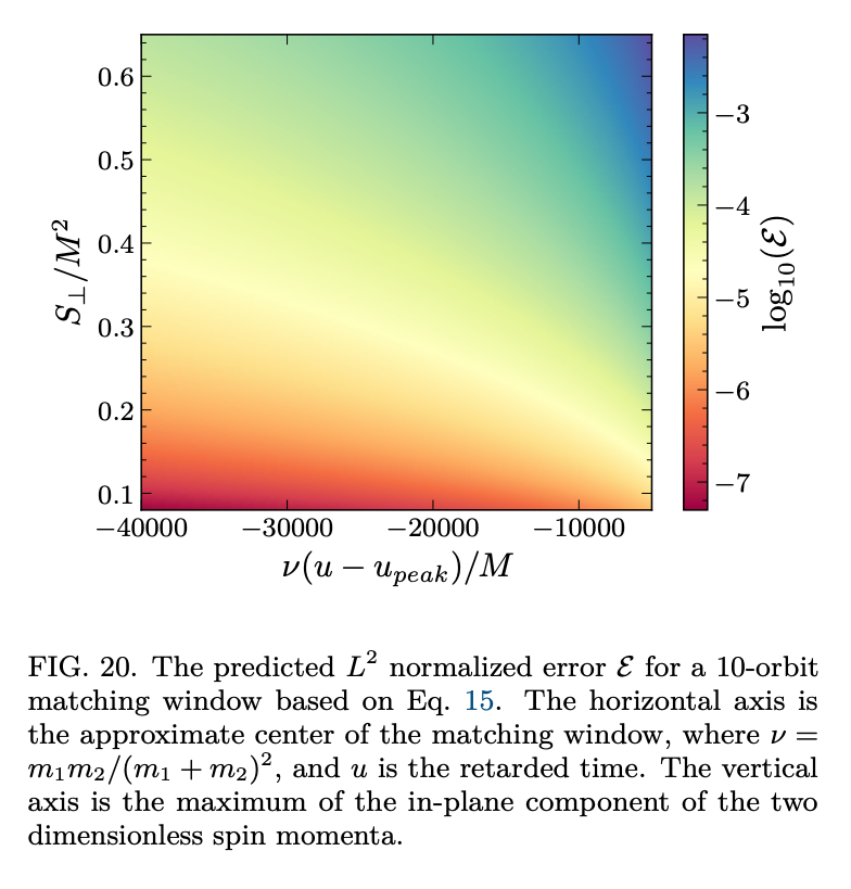
Practitioners probably want to know: Ok, how long should my simulations be? And when should the hybridization window be? For non-precessing systems, there is a balance. Match later and the binary will be more circular. But match earlier and PN does a better job. There is a sweet spot. Meanwhile for precessing systems: We need to go deeper (into the PN regime). Basically, the earlier in time you try to match, the better PN vs NR will agree. This kind of points to needing improvement in precessing PN. You should aim to have at least a full precession cycle in the hybridization window, but that could be longer than most NR simulations!

So, there’s still lots of room for improvement. If we work on modeling eccentric and precessing binaries, we’ll probably be able to do better. And NR simulations should be made longer and more precise, but that costs in CPU time and money! So they need to be more efficient.

If you want to read all the gory details, get them all at [arXiv:2403.10278].