With our latest preprint [arXiv:2412.06887] (led by Marina De Amicis), SXS simulations have for the first time resolved fully nonlinear “tails” from merging black holes. What’s this all about?
First, we have to know something about gravitational waves, or any other massless waves. In flat spacetime with 3 dimensions of space and 1 dimension of time, radiation travels on the surface of the “light cone.” This looks like a 45° line on a spacetime diagram (with c=1)
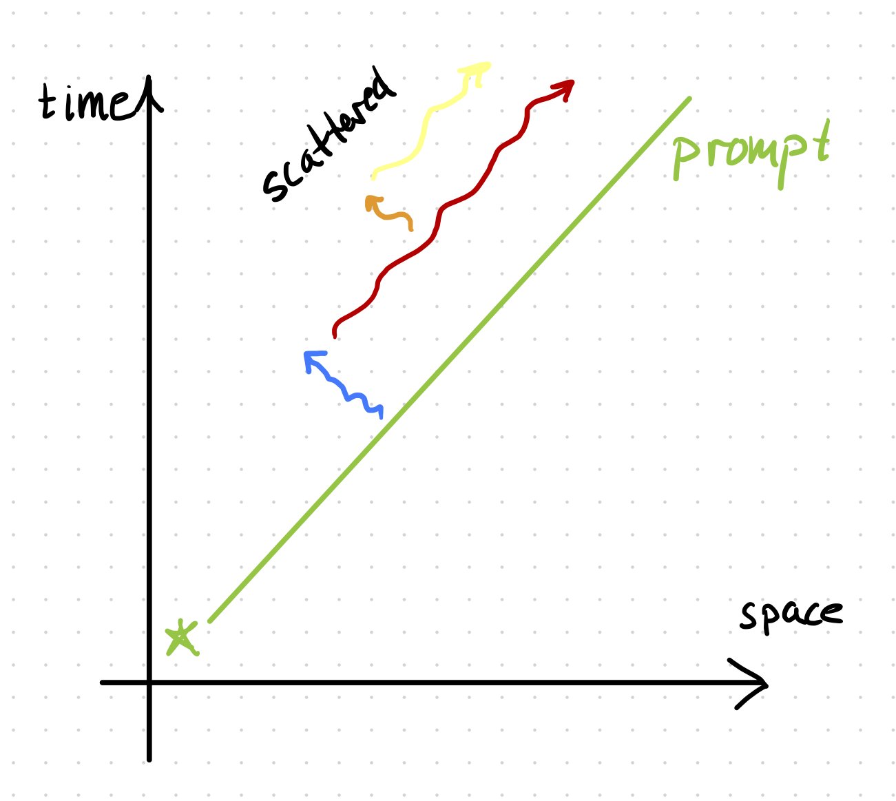
The fact that waves moves only on the surface of the light cone makes it “easy” to figure out what the waves will be far away. You just need to find the intersections between your the sources of waves and your observer’s “past light cone.” That’s just the green curve in the figure.
But curved spacetime changes everything! You can think of curvature as making a scattering potential for light or GWs. Waves interact with curvature, and some of them head off in other directions. Through multiple scatterings, waves fill the interior of the light cone!
Why does this change everything? Instead of just needing to know how sources intersect the observer’s past light cone, we need to know their entire past history — every point in their past history will affect the waves the observer sees at some time!
Alright, back to what this means for gravitational waves we should observe. After black holes smash into each other, we expect the late time signal to be a “ringdown” as the remnant black hole settles down to a stationary state. This is usually modeled as “quasinormal modes.”
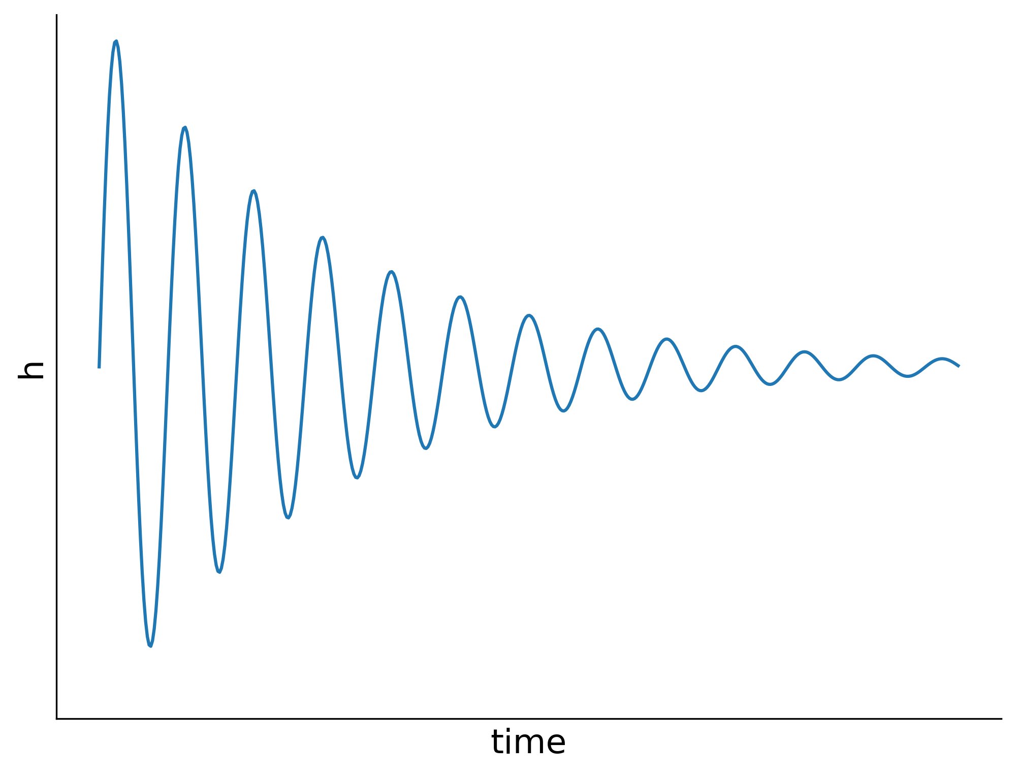
Quasinormal modes are just damped sinusoids. But there is another—much more subtle—component to the late-time signal, that’s due to the back-scattering I was talking about before! That other part is called the “tail.”
The tail is the result of integrating over the whole past history of the source that’s responsible for the GWs. At super late times, it’s roughly like a power law. The important key point is that exponentials decay faster than power laws, so tails will eventually dominate!
Now, tails have been found before—but only by simulating linearized general relativity. Nobody had seen tails in fully non-linear 3+1d numerical relativity simulations — until now! Hopefully you can see one reason why it’s so hard to get these out of the data.
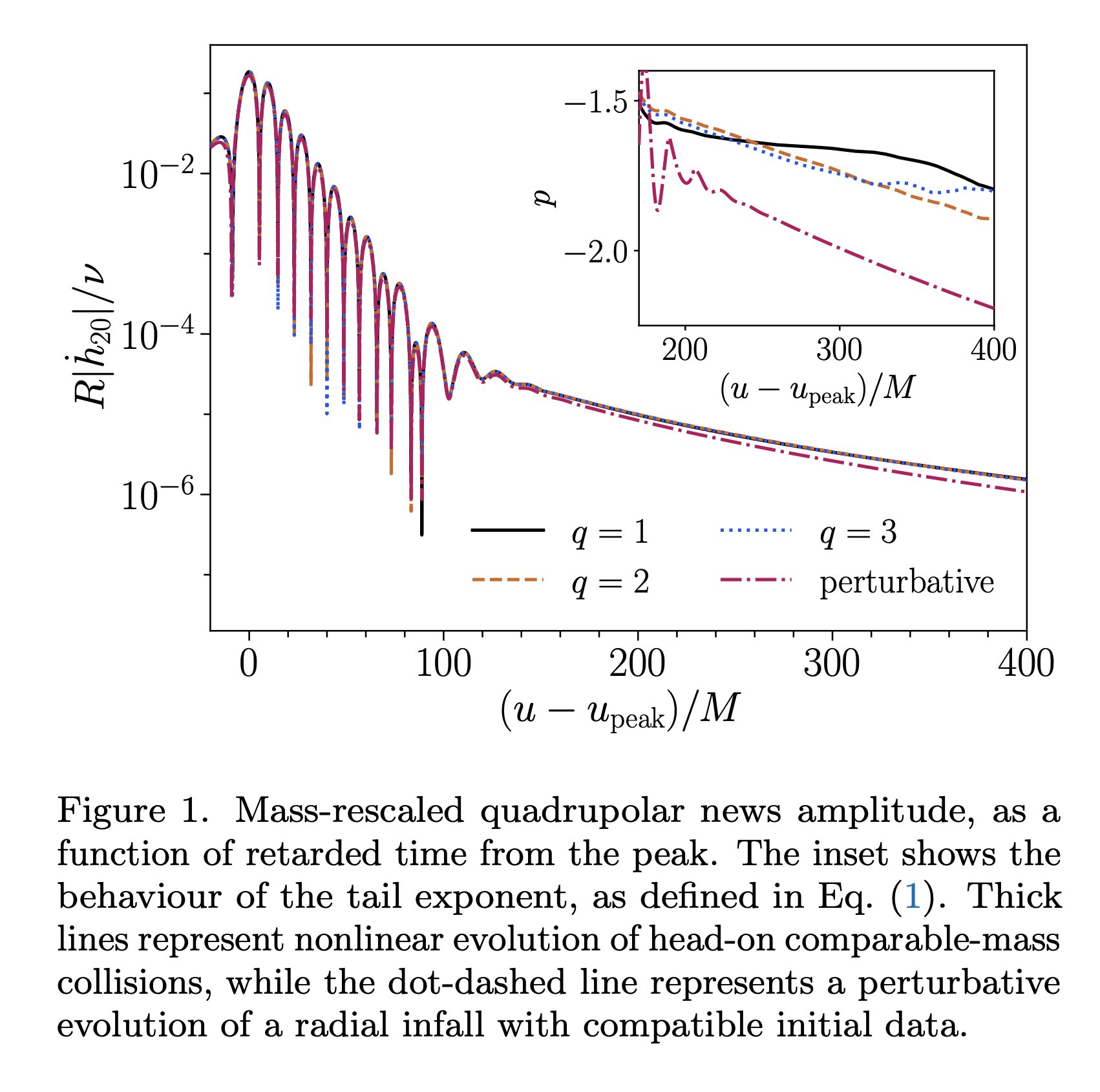
We have to wait a long time for the quasinormal ringing to get quiet enough that it falls below the level of the tail. But that’s not enough. So many things in our simulations could have made a signal that vaguely like a tail. We had to have guidance from analytical theory.
Of course we had to check that our results were independent of numerical resolution, and followed the expected analytical scaling with some parameter we could tune — in our case, the mass ratio of the two black holes. But there were some more key ingredients.
We needed to understand just how far out to put our sim’s outer boundaries. The issue is that our boundary only has approximately correct boundary conditions, which makes scattering that could contaminate the signal we’re looking for. We only want real curvature scattering!
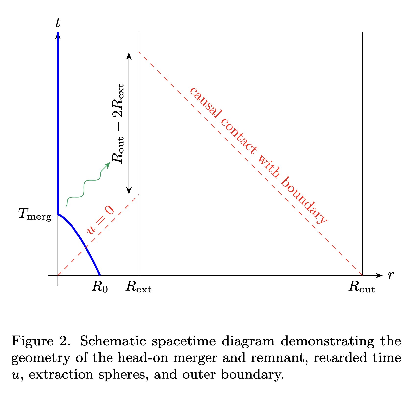
It was also key to understand that the tail is maximized relative to the prompt signal by having mostly radial motion. In our case, we simulated head-on mergers, starting from rest “at infinity.” It’s highly unphysical, but it’s key to seeing the tails.
In the end, this is not observationally relevant (yet!?), but it’s another step along the path of turning gravitational-wave science into a precision field. Hope you enjoyed this tale of tails! If you want all the details, head to [arXiv:2412.06887] and give us a read.